This means that manipulating environmental factors, such as diet and lifestyle, can strongly influence how the traits are finally expressed in humans. But each individual tends to respond differently to diet and lifestyle changes, because each individual is unique in terms of his or her combination of “nature” and “nurture”. Even identical twins are different in that respect.
When plotted, traits that are influenced by our genes are distributed along a bell-shaped curve. For example, a trait like body fat percentage, when measured in a population of 1000 individuals, will yield a distribution of values that will look like a bell-shaped distribution. This type of distribution is also known in statistics as a “normal” distribution.
Why is that?
The additive effect of genes and the bell curve
The reason is purely mathematical. A measurable trait, like body fat percentage, is usually influenced by several genes. (Sometimes individual genes have a very marked effect, as in genes that “switch on or off” other genes.) Those genes appear at random in a population, and their various combinations spread in response to selection pressures. Selection pressures usually cause a narrowing of the bell-shaped curve distributions of traits in populations.
The genes interact with environmental influences, which also have a certain degree of randomness. The result is a massive combined randomness. It is this massive randomness that leads to the bell-curve distribution. The bell curve itself is not random at all, which is a fascinating aspect of this phenomenon. From “chaos” comes “order”. A bell curve is a well-defined curve that is associated with a function, the probability density function.
The underlying mathematical reason for the bell shape is the central limit theorem. The genes are combined in different individuals as combinations of alleles, where each allele is a variation (or mutation) of a gene. An allele set, for genes in different locations of the human DNA, forms a particular allele combination, called a genotype. The alleles combine their effects, usually in an additive fashion, to influence a trait.
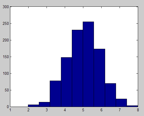
Here is a simple illustration. Let us say one generates 1000 random variables, each storing 10 random values going from 0 to 1. Then the values stored in each of the 1000 random variables are added. This mimics the additive effect of 10 genes with random allele combinations. The result are numbers ranging from 1 to 10, in a population of 1000 individuals; each number is analogous to an allele combination. The resulting histogram, which plots the frequency of each allele combination (or genotype) in the population, is shown on the figure bellow. Each allele configuration will “push for” a particular trait range, making the trait distribution also have the same bell-shaped form.
The bell curve, research studies, and what they mean for you
Studies of the effects of diet and exercise on health variables usually report their results in terms of average responses in a group of participants. Frequently two groups are used, one control and one treatment. For example, in a diet-related study the control group may follow the Standard American Diet, and the treatment group may follow a low carbohydrate diet.
However, you are not the average person; the average person is an abstraction. Research on bell curve distributions tells us that there is about a 68 percentage chance that you will fall within a 1 standard deviation from the average, to the left or the right of the “middle” of the bell curve. Still, even a 0.5 standard deviation above the average is not the average. And, there is approximately a 32 percent chance that you will not be within the larger -1 to 1 standard deviation range. If this is the case, the average results reported may be close to irrelevant for you.
Average results reported in studies are a good starting point for people who are similar to the studies’ participants. But you need to generate your own data, with the goal of “knowing yourself through numbers” by progressively analyzing it. This is akin to building a “numeric diary”. It is not exactly an “N=1” experiment, as some like to say, because you can generate multiple data points (e.g., N=200) on how your body alone responds to diet and lifestyle changes over time.
HealthCorrelator for Excel (HCE)
I think I have finally been able to develop a software tool that can help people do that. I have been using it myself for years, initially as a prototype. You can see the results of my transformation on this post. The challenge for me was to generate a tool that was simple enough to use, and yet powerful enough to give people good insights on what is going on with their body.
The software tool is called HealthCorrelator for Excel (HCE). It runs on Excel, and generates coefficients of association (correlations, which range from -1 to 1) among variables and graphs at the click of a button.
This 5-minute YouTube video shows how the software works in general, and this 10-minute video goes into more detail on how the software can be used to manage a specific health variable. These two videos build on a very small sample dataset, and their focus is on HDL cholesterol management. Nevertheless, the software can be used in the management of just about any health-related variable – e.g., blood glucose, triglycerides, muscle strength, muscle mass, depression episodes etc.
You have to enter data about yourself, and then the software will generate coefficients of association and graphs at the click of a button. As you can see from the videos above, it is very simple. The interpretation of the results is straightforward in most cases, and a bit more complicated in a smaller number of cases. Some results will probably surprise users, and their doctors.
For example, a user who is a patient may be able to show to a doctor that, in the user’s specific case, a diet change influences a particular variable (e.g., triglycerides) much more strongly than a prescription drug or a supplement. More posts will be coming in the future on this blog about these and other related issues.